Quantum Lens - Beginner's Guide
Welcome to Quantum Computing! This guide will help you understand quantum computing concepts from scratch and learn how to use Quantum Lens effectively.
1. Introduction to Quantum Computing
What is Quantum Computing?
Quantum computing uses the principles of quantum mechanics to perform calculations. Unlike classical computers that use bits (0 or 1), quantum computers use qubits that can be in multiple states simultaneously.
Why Does It Matter?
Quantum computers can solve certain problems exponentially faster than classical computers, including:
- Drug discovery and molecular simulation
- Cryptography and security
- Optimization problems
- Machine learning and AI
| Key Differences from Classical Computing | Classical Bit | Qubit |
|---|
| States | Either 0 OR 1 | Can be 0 AND 1 simultaneously |
| Nature | Deterministic | Probabilistic |
| Cloning | Copied easily | Cannot be copied (no-cloning theorem) |
| Measurement | Not affected by measurement | Measurement changes the state |
2. Understanding Qubits
What is a Qubit?
A qubit (quantum bit) is the basic unit of quantum information. Think of it as a coin:
- Classical bit: Coin lying flat (definitely heads or tails)
- Qubit: Coin spinning in the air (both heads AND tails until it lands)
Qubit States
A qubit can be in three types of states:
- Basic States:
- |0⟩ (ket zero): Like "heads" or classical 0
- |1⟩ (ket one): Like "tails" or classical 1
- Superposition State:
- |ψ⟩ = α|0⟩ + β|1⟩: Both 0 and 1 at the same time!
- α and β are complex numbers where |α|² + |β|² = 1
- |α|² = probability of measuring 0
- |β|² = probability of measuring 1
Example: |ψ⟩ = 0.6|0⟩ + 0.8|1⟩
- 36% chance of measuring |0⟩
- 64% chance of measuring |1⟩
Measurement: When you measure a qubit, the superposition collapses to either |0⟩ or |1⟩. You can never see the superposition directly, and measurement is irreversible.
3. Quantum Gates Explained
Quantum gates are operations that change qubit states. Think of them as instructions or commands.
Single-Qubit Gates:
H (Hadamard Gate)
- What it does: Creates superposition
- Use case: Starting point for most quantum algorithms
- Example: H|0⟩ = (|0⟩ + |1⟩)/√2 (equal superposition)
- Visual: Rotates from North pole to equator on Bloch sphere
X (Pauli-X / NOT Gate)
- What it does: Flips the qubit (0↔1)
- Use case: Quantum version of classical NOT gate
- Example: X|0⟩ = |1⟩ and X|1⟩ = |0⟩
- Visual: Rotates 180° around X-axis on Bloch sphere
Y (Pauli-Y Gate)
- What it does: Flips qubit AND adds phase
- Use case: Combined bit-flip and phase-flip
- Example: Y|0⟩ = i|1⟩ and Y|1⟩ = -i|0⟩
- Visual: Rotates 180° around Y-axis on Bloch sphere
Z (Pauli-Z Gate)
- What it does: Flips the phase (sign) of |1⟩
- Use case: Phase manipulation without changing probabilities
- Example: Z|0⟩ = |0⟩ and Z|1⟩ = -|1⟩
- Visual: Rotates 180° around Z-axis on Bloch sphere
S (Phase Gate)
- What it does: Adds 90° phase shift
- Use case: Quarter rotation for fine phase control
- Example: S|1⟩ = i|1⟩
- Visual: Rotates 90° around Z-axis on Bloch sphere
T (π/8 Gate)
- What it does: Adds 45° phase shift
- Use case: Precise phase control, universal gate set
- Example: T|1⟩ = e^(iπ/4)|1⟩
- Visual: Rotates 45° around Z-axis on Bloch sphere
I (Identity Gate)
- What it does: Does nothing (leaves qubit unchanged)
- Use case: Timing, keeping qubits idle
- Example: I|ψ⟩ = |ψ⟩
- Visual: No movement on Bloch sphere
Two-Qubit Gates:
CNOT (Controlled-NOT)
- What it does: Flips target qubit IF control qubit is |1⟩
- Use case: Creating entanglement
- Example:
- Control=|0⟩, Target=|0⟩ → |00⟩ (nothing happens)
- Control=|1⟩, Target=|0⟩ → |11⟩ (target flips)
- Key feature: This is THE gate for creating entanglement!
4. Building Your First Circuit
Step-by-Step Tutorial:
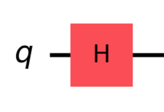
Circuit 1: Simple Superposition
What happens:
- Qubit starts in |0⟩
- Hadamard creates superposition: (|0⟩+|1⟩)/√2
- Measurement gives 50% chance of 0, 50% chance of 1
Try in Quantum Lens:
- Add a qubit
- Drag Hadamard gate to the qubit
- Run with 1000 shots
- Observe the Bloch sphere - qubit is on the equator!
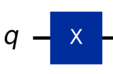
Circuit 2: Bit Flip
What happens:
- Qubit starts in |0⟩
- X gate flips it to |1⟩
- Measurement gives 100% chance of 1
Try in Quantum Lens:
- Add a qubit
- Drag X gate
- Observe Bloch sphere - qubit moves from North to South pole!
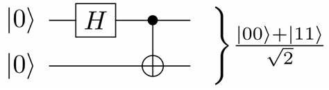
Circuit 3: Bell State (Entanglement!)
What happens:
- H creates superposition on q0: (|0⟩+|1⟩)/√2
- CNOT entangles both qubits
- Final state: (|00⟩+|11⟩)/√2 (Bell state)
- Qubits are now connected - measuring one affects the other!
Try in Quantum Lens:
- Add 2 qubits
- Apply H to qubit 0
- Apply CNOT (control=0, target=1)
- Look at both Bloch spheres - both qubits are now INSIDE the sphere (mixed states!)
- This proves entanglement!
5. Understanding the Bloch Sphere
What is Bloch Sphere
The Bloch sphere is a 3D visualization of a single qubit's quantum state. It's like a globe representing all possible qubit states.
Key Features:
The Poles:
- North Pole (top): |0⟩ state
- South Pole (bottom):|1⟩ state
The Equator:
- +X axis:|+⟩ = (|0⟩+|1⟩)/√2
- -X axis:|-⟩ = (|0⟩-|1⟩)/√2
- +Y axis:|+i⟩ = (|0⟩+i|1⟩)/√2
- -Y axis: |-i⟩ = (|0⟩-i|1⟩)/√2
Position Meaning:
- On the Surface (Pure States):
- The qubit is in a definite quantum state
- Radius = 1
- Complete quantum information
- Inside the Sphere (Mixed States):
- The qubit is uncertain or entangled
- Radius < 1
- Lost some quantum information
- At the Center (Maximally Mixed):
- Complete uncertainty (50-50 chance of 0 or 1)
- Radius = 0
- No quantum information left
Reading the Bloch Sphere:
Coordinates (x, y, z):
- x-coordinate:Measures superposition in X direction
- y-coordinate: Measures superposition in Y direction
- z-coordinate: Measures probability (z=1 means |0⟩, z=-1 means |1⟩)
Distance from center:
- Shows "purity" of the state
- Pure state = on surface
- Mixed state = inside
6. What is Entanglement?
Simple Explanation: Entanglement is when two or more qubits become connected so that measuring one instantly affects the others, no matter how far apart they are.
The Magic:
Imagine two magic coins:
- You flip both together using special quantum magic
- They fly to opposite ends of the universe
- When you check one coin and it's heads, the other is INSTANTLY heads too
- When you check one and it's tails, the other is INSTANTLY tails too
- They're always synchronized, even though they're far apart!
Real Example - Bell State:
State: (|00⟩+|11⟩)/√2
What this means:
- Both qubits are in superposition
- They're correlated: both will be 0 OR both will be 1
- You won't know which until you measure
- But they'll ALWAYS match!
How to Create Entanglement:
- Put first qubit in superposition (H gate)
- Apply CNOT to link them together
- Now they're entangled!
Detecting Entanglement in Quantum Lens:
Look at the Bloch spheres:
- Entangled qubits: Both appear INSIDE the sphere (mixed)
- Not entangled: Both on the surface (pure)
Even though the overall state is pure, individual qubits look mixed when entangled!
7. Density Matrices and Mixed States
What is a Density Matrix?
A density matrix is a mathematical way to describe quantum states, especially when they're mixed or uncertain.
Why Use Density Matrices?
- State vectors (|ψ⟩) only work for pure states
- Density matrices (ρ) work for BOTH pure and mixed states
- Essential for understanding individual qubits in entangled systems
Pure vs Mixed States:
Pure State:
- Complete quantum information
- Can be written as |ψ⟩
- Density matrix: ρ = |ψ⟩⟨ψ|
- Purity: Tr(ρ²) = 1
- On Bloch sphere: On the surface
Mixed State:
- Incomplete information or entangled with others
- Cannot be written as single |ψ⟩
- Density matrix: ρ = Σ pᵢ|ψᵢ⟩⟨ψᵢ|
- Purity: Tr(ρ²) < 1
- On Bloch sphere: Inside the sphere
Example:
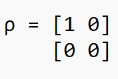
Pure state |0⟩:
Tr(ρ²) = 1 ✓ Pure
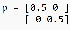
Maximally mixed state:
Tr(ρ²) = 0.5 ✘ Mixed
8. Partial Trace Explained
What is Partial Trace?
Partial trace is the mathematical operation that lets us focus on one qubit while "ignoring" or "tracing out" the others.
Why Do We Need It?
When qubits are entangled, you can't describe one qubit independently. Partial trace gives us the reduced density matrix - the best description of a single qubit's state.
The Problem:
You have a 2-qubit entangled state: (|00⟩+|11⟩)/√2
Question: What is the state of just qubit 1?
You might think: "It's (|0⟩+|1⟩)/√2"
But that's WRONG! Because qubit 1 is entangled, it doesn't have a pure state on its own.
The Solution - Partial Trace:
When we trace out qubit 2, we get:
This is a maximally mixed state - qubit 1 appears completely random!
Key Insight:
Entanglement makes individual qubits appear mixed, even though the total system is pure.
In Quantum Lens:
Our tool automatically performs partial trace for each qubit and shows you:
- The reduced density matrix
- The state on the Bloch sphere
- Whether it's pure (surface) or mixed (inside)
9. Understanding Circuit Metrics
Circuit Depth
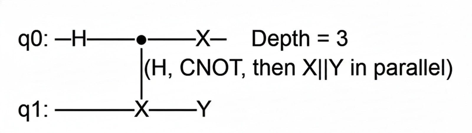
What it is: The number of sequential time steps needed to execute the circuit.
Why it matters:
- Lower depth = Better for real quantum hardware
- Qubits decohere over time - deep circuits may fail
- Each layer adds time for errors to accumulate
Example:
In Quantum Lens: We show circuit depth so you can optimize your quantum algorithms for real hardware.
Shots (Measurements)
What it is: The number of times you run the quantum circuit.
Why it matters:
- Quantum measurements are probabilistic
- More shots = more accurate statistics
- Fewer shots = faster but noisier results
Example: If true probability is 30% for |0⟩:
- 10 shots: Might see 2 or 4 (inaccurate)
- 100 shots: See around 28-32 (better)
- 1000 shots: See around 295-305 (very accurate)
In Quantum Lens: Adjust shots to balance speed vs accuracy:
- 100-500 shots: Quick testing
- 1000-5000 shots: Standard accuracy
- 10000+ shots: High precision
10. Tips and Best Practices
For Beginners:
- Start Simple
- Begin with 1-2 qubits
- Use basic gates (H, X, Z)
- Gradually add complexity
- Visualize Everything
- Always check the Bloch sphere
- Watch how gates change the state
- Compare before and after
- Experiment!
- Try different gate combinations
- See what creates entanglement
- Learn by doing
- Use Enough Shots
- Start with 1000 shots
- Increase if results look noisy
- Remember: more shots = more accurate
What is Noise in Quantum Computing?
Noise is unwanted interference that corrupts quantum information, causing errors in quantum computations. It's the biggest challenge in building practical quantum computers.
Simple Explanation:
Think of qubits like extremely delicate instruments playing music:
- Perfect quantum state: Beautiful, clear note
- Noise: Static, interference, vibrations that distort the sound
- Result: The music (quantum computation) gets corrupted
11. Types of Noise
1. DEPOLARIZATION NOISE
What It Is: The qubit randomly flips to a completely random state. It's like the qubit "forgets" what state it was in and becomes completely mixed.
What Happens:
- With probability p, the qubit gets replaced by a maximally mixed state (center of Bloch sphere)
- The qubit applies random X, Y, or Z errors
- Effect: Bloch vector shrinks toward the center
Physical Cause:
- Random interactions with environment
- Loss of quantum information to surroundings
- General "quantum noise"
Example:
- 0.00 (No noise): Qubit stays pure, on Bloch sphere surface
- 0.10 (10% noise): Bloch vector at 90% of original length
- 0.30 (30% noise): Bloch vector at 70% of original length
- 1.00 (100% noise): Qubit completely at center (totally random)
In our Tool: As you increase depolarization from 0.00 to 0.30, you will see the Bloch vector shrink.
- Pure states move toward center
- Superposition becomes "fuzzier"
- Measurement outcomes become more random
2. T1 AMPLITUDE DAMPING
What It Is:
The qubit loses energy and decays toward the |0⟩ state. It's like a ball rolling downhill - it naturally wants to settle at the ground state.
What Happens:
- The qubit gradually relaxes from |1⟩ toward |0⟩
- |1⟩ is unstable and decays
- |0⟩ is stable and doesn't decay
- Effect: Bloch vector moves toward North pole (|0⟩)
Physical Cause:
- Energy loss to the environment
- Spontaneous emission
- Thermal relaxation
T1 Time:
The "T1" refers to the characteristic decay time. T1 might be 50-100 microseconds on real hardware.
Example:
Start with |1⟩ state:
- 0.00 (No noise): Stays at |1⟩ (South pole)
- 0.10 (10% damping): Slightly moves toward |0⟩
- 0.30 (30% damping): Significantly closer to |0⟩
- 1.00 (100% damping): Completely decayed to |0⟩
In our Tool:
As you increase T1 amplitude damping from 0.00 to 0.30:
- States drift toward North pole (|0⟩)
- Excited state |1⟩ becomes harder to maintain
- Measurements show more |0⟩ outcomes than expected
3. T2 PHASE DAMPING
What It Is:
The qubit loses phase information but NOT energy. The probabilities of |0⟩ and |1⟩ stay the same, but the quantum phase gets randomized.
What Happens:
- Superposition states lose coherence
- No change in z-coordinate (probabilities unchanged)
- x and y coordinates shrink (phase randomizes)
- Effect: Bloch vector moves toward Z-axis
Physical Cause:
- Random phase fluctuations
- Magnetic field noise
- Low-frequency environmental fluctuations
T2 Time:
The "T2" is the dephasing time. Always T2 ≤ 2×T1 in real systems.
Example:
Start with |+⟩ = (|0⟩+|1⟩)/√2 on +X axis:
- 0.00 (No noise): Stays on equator at +X
- 0.10 (10% dephasing): Moves slightly toward Z-axis
- 0.30 (30% dephasing): Significantly closer to Z-axis
- 1.00 (100% dephasing): On Z-axis (classical mixture, no phase coherence)
In our Tool:
As you increase T2 phase damping from 0.00 to 0.30:
- Horizontal (XY) components shrink
- Vertical (Z) component unchanged
- Superposition "collapses" but probabilities stay same
4. |0⟩ → |1⟩ READOUT ERROR
What It Is:
When the TRUE state is |0⟩, but the measurement incorrectly reads |1⟩.
What Happens:
- False positive: Detector says "1" when it should say "0"
- Probability: The number you set (e.g., 0.30 = 30% error rate)
- Doesn't affect the quantum state, only the measurement outcome
Physical Cause:
- Detector imperfections
- Thermal excitations during readout
- Timing errors in measurement pulse
Example:
- 0.00 (Perfect): Measuring |0⟩ always gives 0
- 0.10 (10% error): Measuring |0⟩ gives 1 about 10% of the time
- 0.30 (30% error): Measuring |0⟩ gives 1 about 30% of the time
In our Tool:
If true state is 100% |0⟩:
- 0.00 error: Histogram shows 100% |0⟩, 0% |1⟩ ✓
- 0.30 error: Histogram shows 70% |0⟩, 30% |1⟩ (30% wrong!)
5. |1⟩ → |0⟩ READOUT ERROR
What It Is:
When the TRUE state is |1⟩, but the measurement incorrectly reads |0⟩.
What Happens:
- False negative: Detector says "0" when it should say "1"
- Probability: The number you set
- Measurement error only
Physical Cause:
- Insufficient readout signal
- Decay during measurement
- Readout pulse timing
Example:
- 0.00 (Perfect): Measuring |1⟩ always gives 1
- 0.10 (10% error): Measuring |1⟩ gives 0 about 10% of the time
- 0.30 (30% error): Measuring |1⟩ gives 0 about 30% of the time
In our Tool:
If true state is 100% |1⟩:
- 0.00 error: Histogram shows 0% |0⟩, 100% |1⟩ ✓
- 0.30 error: Histogram shows 30% |0⟩, 70% |1⟩ (30% wrong!)
WHAT HAPPENS WHEN YOU INCREASE ALL NOISE TO 0.30?
Let me show you with a concrete example:
Example Circuit: Bell State
IDEAL (All noise = 0.00):
States:
- Both qubits: Maximally mixed (center of Bloch sphere)
- Perfectly entangled
Measurements:
- 50% |00⟩
- 50% |11⟩
- 0% |01⟩
- 0% |10⟩
Bloch Sphere:
- Both qubits exactly at center
- Perfect entanglement signature
WITH ALL NOISE = 0.30:
1. Depolarization (0.30):
- Adds random errors throughout circuit
- States become "fuzzier"
- Some entanglement is lost
2. T1 Amplitude Damping (0.30):
- Both qubits drift toward |0⟩
- More |00⟩ outcomes than expected
- Asymmetry appears
3. T2 Phase Damping (0.30):
- Phase coherence is lost
- Interference effects weaken
- Superposition partially destroyed
4. Readout Errors (0.30 each):
- 30% of |0⟩ reads as |1⟩
- 30% of |1⟩ reads as |0⟩
- Completely messes up measurement statistics
COMBINED RESULT:
States on Bloch Sphere:
- NOT at exact center anymore
- Slightly toward North pole (due to T1)
- Smaller radius (due to depolarization and T2)
- Less pure than ideal
Measurements (approximate):
- ~55% |00⟩ (should be 50%, but T1 bias + readout errors)
- ~25% |11⟩ (should be 50%, reduced by noise)
- ~10% |01⟩ (should be 0%, readout errors!)
- ~10% |10⟩ (should be 0%, readout errors!)
What You'd See:
- Histogram bars NOT clean (should only be |00⟩ and |11⟩)
- Wrong ratios
- Unexpected outcomes
- Bloch vectors slightly off-center and biased toward |0⟩
Quantum Circuit Simulator: Execution Flow and Qiskit Components
This simulator builds a Qiskit QuantumCircuit from the user-placed gates and then runs it to produce a circuit diagram, measurement outcomes, and per-qubit state analyses. When Execute is clicked, the app follows these steps: (1) Build the circuit by reading the gate grid and appending gates to a QuantumCircuit, (2) Visualize it using qc.draw(), (3) Simulate measurements with Qiskit Aer, producing a counts histogram, and (4) Analyze the final quantum state, computing each qubit's reduced density matrix and Bloch vector. Below we detail each stage, citing how Qiskit's components work under the hood.
Circuit Construction (QuantumCircuit)
- Reading the gate grid: The app maintains
st.session_state.circuit_grid, a list-of-lists representing qubits vs. time steps. On execution, it creates an empty QuantumCircuit(num_qubits) and loops over each time step. It looks for '●' (CNOT control) and '⊕' (CNOT target) symbols. If both are found in a column, it calls qc.cx(control, target) to append a CNOT gate; if only one appears, it raises an error (an incomplete CNOT). If no CNOT is present in that time slot, it applies single-qubit gates: e.g. if the grid has 'H' at qubit q, time t, it does qc.h(q). Each call like qc.h(q) or qc.x(q) appends an instruction to the circuit's internal data. Internally, QuantumCircuit holds a list qc.data of CircuitInstruction objects; each instruction node contains the gate and its target qubits. In fact, Qiskit builds a Directed Acyclic Graph (DAG) of these instructions so that later optimizations/transpilation can occur, though this app does not explicitly transpile.
- Internal representation: For example, after calling
qc.x(0) on an empty 2-qubit circuit, qc.data becomes a list containing one CircuitInstruction whose operation is the X-gate and whose qubits=(q0,). In general, each gate method (.h(), .cx(), etc.) mutates the circuit by adding that gate to qc.data. Thus by the end of this step, the Qiskit circuit holds exactly the sequence of gates the user placed.
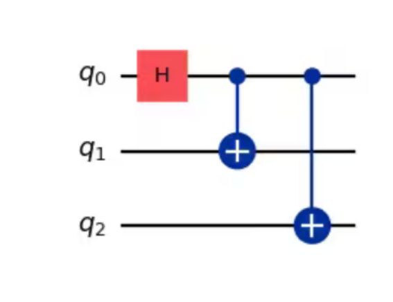
from qiskit import QuantumCircuit
# Create a circuit with a register of three qubits
circ = QuantumCircuit(3)
# H gate on qubit 0, putting this qubit in a superposition of |0> + |1>.
circ.h(0)
# A CX (CNOT) gate on control qubit 0 and target qubit 1 generating a Bell state.
circ.cx(0, 1)
# CX (CNOT) gate on control qubit 0 and target qubit 2 resulting in a GHZ state.
circ.cx(0, 2)
# Draw the circuit
circ.draw('mpl')
The above code will give us the circuit diagram:
Execution Workflow of the Quantum Circuit Simulator
- Gate Placement (UI Interaction): The user selects gates in the sidebar and clicks cells on the grid. Each click calls the
place_gate(q,t) callback, which records the active gate symbol (e.g. H, X, ● for a CNOT control, ⊕ for a target) into the 2D grid st.session_state.circuit_grid. This grid is a Python list-of-lists indexed by qubit (row) and time-step (column). A special two-step logic handles CNOT gates: first a control ● is placed (setting active_gate to ⊕), then a target ⊕ is placed at another row. Internally this updates the grid state and also pushes a snapshot of the grid onto an undo stack (via save_to_history()) for undo/redo support. Each cell's content (gate symbol) is ultimately just a string in the grid.
- Constructing the Qiskit QuantumCircuit: When Execute is clicked, the code builds a new
QuantumCircuit(num_qubits) object (no classical bits needed until measurement). It then iterates through each time step (column) and qubit (row) to apply the gates from the grid into the QuantumCircuit. In each column it first checks for a CNOT: it scans for a control ● and a target ⊕. If both are found, it applies qc.cx(control, target) (the CNOT instruction). If only one of ● or ⊕ is present, it throws an error ("Incomplete CNOT") to avoid inconsistent gates. Otherwise, for each qubit it sees a single-qubit gate symbol (H, X, Y, Z, S, T), it calls the corresponding Qiskit method: for example, qc.h(q) for a Hadamard on qubit q, or getattr(qc, gate.lower())(q) for generality. Each call like qc.x(0) appends an Instruction to the circuit's internal list (qc.data). As Qiskit notes, "adding an instruction to the circuit appends the instruction to the circuit's data attribute". Thus by the end of this loop, the code has built up a full QuantumCircuit object representing exactly the user-designed circuit. (Optionally, one could transpile the circuit to optimize it or target a specific device, but this demo code directly uses the built circuit.)
Figure: Example multi-qubit circuit diagram as drawn by Qiskit. Once the QuantumCircuit is
built, the code produces a visual diagram. Calling qc.draw(output='mpl') uses Matplotlib
to render a gate-by-gate circuit diagram. Qiskit’s documentation explains that qc.draw()
returns this diagram (by default as ASCII, or as a Matplotlib figure when mpl is specified). For
example, a 5-qubit circuit might be visualized as shown above. In this image, each row is a qubit
(labeled q[0] through q[4]), horizontal lines are wire timelines, and gate symbols (H, X, U1, etc.)
are placed in time order. Vertical lines connect multi-qubit gates (like CNOT or
controlled-phase). This diagram is generated just before measurement and saved as a plot that
Streamlit displays.
- Adding Measurements and Running the Simulation: Before simulating, the code appends a measurement on every qubit by calling
qc_measured = qc.copy(); qc_measured.measure_all(). This adds measurement instructions mapping each quantum bit to a classical bit. The circuit is now complete with all gates and measurements.
- Ideal (Noiseless) Simulation: The code uses Qiskit Aer's qasm_simulator to perform a shot-based simulation. It obtains the backend via
Aer.get_backend('qasm_simulator'), then runs the circuit with a specified number of shots. The simulator samples the circuit many times: each "shot" executes the entire circuit on a virtual quantum register, collapsing to a classical outcome. The result is an object from which we call result.get_counts(). This returns a dictionary mapping bitstrings to occurrence counts. Qiskit docs note that "the basic operation runs a quantum circuit and returns a counts dictionary of measurement outcomes". For example, if result.get_counts() returns {'010' : 512, '110' : 256, '000' : 256}, it means 010 occurred 512 times, etc.
- Most Probable Outcome: The code finds the key with the maximum count using
max(counts, key=counts.get). This identifies the bitstring with the highest frequency, which is reported as the "Most Probable Classical Outcome." For instance, if counts = {'00': 800, '11': 200}, the most likely is '00'.
- Bit-String Ordering: It's important to interpret the bitstrings correctly. Qiskit uses little-endian ordering by default: the rightmost bit in the string is qubit q0, next is q1, and so on. (This code makes this explicit in a help message: "bit string is ordered from highest to lowest qubit index... Qubit q0 is rightmost.") In the example above, the string '010' means q2=0 (leftmost), q1=1, q0=0 (rightmost). As the Qiskit API docs explain, the count dictionary keys are binary strings with qubit 0 on the right side.
- Displaying Results: The code then visualizes the measurement histogram using Plotly and also shows the raw counts. This completes the classical outcome part of the workflow.
- Noise Model (Optional): If "Enable Simulation Noise" is checked, the code injects a custom noise model into the simulation. It constructs a NoiseModel (from
qiskit_aer.noise) and adds specified errors. For example, depolarizing_error(p, 1) creates a single-qubit depolarizing channel with probability p; amplitude_damping_error(gamma) and phase_damping_error(gamma) create relaxation errors. Each is added to all single-qubit gates via noise.add_all_qubit_quantum_error(...). Similarly, a readout error is added via ReadoutError ([[1-p01, p01], [p10, 1-p10]]) for imperfect measurement. In Qiskit Aer, a NoiseModel can store such gate and readout errors and the simulator will randomly apply them during each shot, emulating a noisy quantum device.
- Ideal State Analysis (Density Matrix & Bloch Spheres): In addition to the classical outcomes, the code also computes the theoretical quantum state just before measurement. It does this using a state-vector/density-matrix simulator. Specifically, it uses AerSimulator(method='density_matrix') (including the same noise model if enabled) to capture the final density matrix ρ of the full system. By appending
qc_dm.save_density_matrix(), the circuit instructs Aer to record the final state ρ as a density matrix rather than only sampling measurements. After dm_simulator.run(qc_dm).result(), we extract dm = DensityMatrix(result.data(0)["density_matrix"]). This Qiskit DensityMatrix object represents the full N-qubit mixed state.
- Per-Qubit Reduction: To visualize individual qubits, the code takes partial traces: for each qubit index i, it traces out (sums over) all other qubits. This is done via
quantum_info.partial_trace(dm, q_list), yielding a 2×2 reduced density matrix for qubit i. By definition, the Bloch-vector of a single qubit ρ is given by its expectation values of the Pauli matrices:
- Partial Trace → reduced state → Pauli expectations → Bloch vector
- Code Example:
from qiskit.quantum_info import partial_trace, DensityMatrix, Pauli
import numpy as np
rho_i = partial_trace(dm, q_list) # 2x2 reduced state
sx = Pauli('X').to_matrix()
sy = Pauli('Y').to_matrix()
sz = Pauli('Z').to_matrix()
x = np.trace(rho_i.data @ sx).real
y = np.trace(rho_i.data @ sy).real
z = np.trace(rho_i.data @ sz).real
bloch_vector = np.array([x, y, z])
The above code bloch_vector will be used in plotting of the bloch vector
These are computed from the matrix elements of the 2×2 reduced ρ. Intuitively, (x,y,z) gives the
point on or inside the Bloch sphere representing the qubit’s state. The code also extracts the
diagonal entries as probabilities prob0 = ρ[0,0], prob1 = ρ[1,1], and computes purity =
Tr(ρ²) (which is 1 for a pure state, <1 if mixed).
- Bloch Sphere Visualization: The final step is visualizing these per-qubit states as Bloch spheres. Each qubit's Bloch vector (x,y,z) is plotted on a unit sphere. Qiskit's visualization describes that the axes labeled X,Y,Z on a Bloch sphere correspond to the expected values of Pauli X, Y, Z on that qubit. In other words, the arrow drawn from the origin to the surface point (x,y,z) represents the qubit state (pure states lie on the surface, mixed inside).
MAIN summary
Summary of Execution Flow:
- User places gates on a grid (handled by place_gate).
- On Execute:
- Build a QuantumCircuit and append all gates in order.
- Visualize the circuit with qc.draw().
- Attach measurements (measure_all) and run QASM simulation (with noise if enabled) to get outcome counts.
- Compute and report the highest-frequency bitstring (most likely outcome).
- If noise is on, incorporate the Aer NoiseModel (depolarizing, damping, readout errors) during simulation.
- Separately, run a density-matrix simulation (save_density_matrix) to get the ideal pre-measurement state.
- For each qubit, do a partial trace to get its reduced 2×2 state. Compute its Bloch vector (⟨X⟩,⟨Y⟩,⟨Z⟩), probabilities, and purity.
- Display each qubit's Bloch sphere and statistics.
This completes the program's workflow from interactive gate placement all the way to final visualization. The user's gates become Qiskit instructions, the circuit is drawn, the simulator returns classical outputs (histogram and most-likely bitstring) and quantum states (Bloch spheres), and everything is explained with the conventions (like bitstring ordering) made explicit.
 Quantum Lens